Visualization Tools
PHD2 provides numerous visualization and
display tools to help you see how your guider is performing.
All
of these tools are accessed under the 'View' pull-down menu and are described below.
Overlays
The
simplest display tools are grid overlays superimposed over the
main guider display window. These are quite straightforward
and
include the following choices:
- Bullseye target
- Fine grid
- Coarse grid
- RA/Dec - this shows how the telescope axes are aligned
relative to the axes of the camera sensor
- Spectrograph
slit/slit position - for spectroscopy users, this will overlay a
spectrograph slit graphic on the main display window. The size,
position, and angle of the graphic can be adusted to match the
optical configuration.
- None
You can just click on the various overlay options under the 'View' menu
and choose one that suits you.
Graphical Display
The
graphical display window is one of the more powerful tools for judging
guiding performance, and you will probably learn to rely on it.
A typical example is shown below:
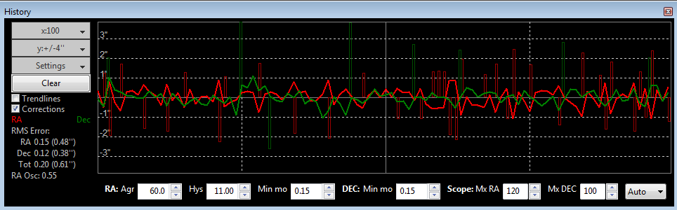
The
major portion of the window shows the detailed displacements of the
guide star for each guide exposure, plotted left-to-right.
Normally, one line shows displacements in right ascension while
the second line shows declination displacements. However, you can
use the 'Settings' button to the left of the graph to switch to camera
(X/Y) axes if you prefer. You can also use the 'Settings' button
to switch between display units of arc-seconds vs. camera pixels or to
change the colors of the two graph lines. The range of the
vertical axis is controlled by the second button from the top, labelled
y:+/-4" in this example. The range of the horizontal axis - the
number of guide exposures being plotted - is controlled by the
topmost button, labelled x:100 in this example. This scale also
controls the sample size used for calculating the
statistics you see in the lower left part of the graph window.
These values show the root-mean-square (RMS or standard
deviation) of the motions in each axis along with the total for both
axes. These are probably your best estimators of guiding
performance because they can be directly compared to star sizes and
seeing conditions. The 'RA Osc' value shows the odds that
the current RA move is in the opposite direction as the last RA move.
If you are too aggressive in your guiding and over-shooting the
mark each time, this number will head toward 1.0. If you were
perfect and not over- or under-shooting and your mount had no periodic
error, the score would be 0.5 Taking periodic error into account,
the ideal value would be closer to 0.3. If this score gets very
low (e.g. 0.1), you may want to increase the RA aggressivness or
decrease the hysteresis. If it gets quite high (e.g. 0.8), you
may want adjust aggressivness/hysteresis in the opposite
direction. There are two
other checkboxes to the left that can help you evaluate guider
performance. Clicking on the 'Corrections' box results in an
overlay showing when guide commands are actually sent to the mount,
along with their direction and magnitude. In this example, these
are shown as the vertical red and green lines appearing at irregular
intervals along the horizontal axis. This shows you how "busy"
the guiding is - under optimal conditions, you should expect to see
extended intervals when no guide commands are sent at all. The
other checkbox, labelled 'Trendlines',
will superimpose trend lines in
both axes to show if there is a consistent overall drift in the star
position. This is primarily useful for drift aligning where the
declination trendline is used extensively. But the RA trendline
can show if your mount is tracking systematically slow or fast (or is
seeing the effects of flexure) and can
help if you are trying to set up custom tracking rates. If
dithering commands are issued, usually by an external imaging
application, a 'dithering' label will be superimposed on the graph in
the appropriate time interval. This tells you that the star
displacements being graphed are being influenced by the dithering
operation.
The recommended way to look at guiding
performance is to use units of arc-seconds rather than pixels.
Doing this allows an equipment-independent way of evaluating
performance because it transcends questions of focal length and image
scale. To do this, you need to provide PHD2 with sufficient
information to determine your guider image scale: namely, the focal
length of the guide scope and the size of the guide camera pixels.
These parameters are set in the 'Brain' dialog, on the 'Global'
and 'Camera' tabs, respectively. If they are not specified, PHD2
will use default values of 1.0, and the guiding performance numbers
will effectively be reported in units of pixels.
At
the bottom
of the graph window are active controls for adjusting guiding
parameters "on the fly". The guiding algorithm selections you've
made will control which controls are shown. These controls have
the same
effect as those in the 'Brain' dialog, and they eliminate the
need to stop guiding and navigate to another window to adjust
guiding parameters.
Stats
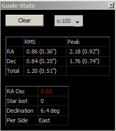
If
you want to monitor guiding performance without necessarily having the
graph window open, you can click on the "Stats" menu item.
That will display the salient statistics with controls for
clearing the data or changing the number of guide exposures used to
compute the statistics.
Star Profile and Target Displays
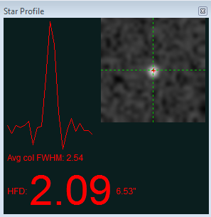
The
star profile display shows the cross-section of the guide star along
with measurements for its full-width-half-maximum (FWHM)
and half-flux-diameter (HFD).
HFD is generaly a more stable measure of the star size since
it doesn't require curve fitting or any assumption about the overall
shape of the star image. That's why automated focusing
applications like FocusMax use it. If you
see substantial fluctuations in this parameter or wildly varying star
profiles, it may be an indication
that the star is too faint or the exposure time is too short.
This tool can also help with focusing the
guide camera, a
procedure that can be a bit tedious if you're using an off-axis-guider
at a fairly long focal length. For that purpose, the HFD number
is shown in a large font so you can see it from a distance while
focusing your guide scope/camera. Just un-dock the Star Profile
window and expand it until you can see the HFD number easily. If
you are starting well out-of-focus, you'll probably see only a few
fuzzy stars in the frame, so just choose the smallest one that is
clearly visible. Use exposure times of at least 2 seconds if
possible so you don't chase the seeing. At the same time, don't
let the star become saturated, showing a distinctive flat top.
Now adjust the focus so the HFD gets consistently
smaller - but stop as soon as HFD reverses direction or seems to
plateau. At that point, the star may be saturated, so move to a
dimmer star in the field. Since you have already improved the
focus, you can hopefully see a dimmer star. Continue in this way
until you've reached a focus point that shows a minimum level of HFD
for the faintest star you can use. At each point in the focusing
process, you'll probably want to watch the HFD values for a few frames
so you can mentally average out the effects of seeing. Bad
focus is a common issue for beginners, leading to problems in
calibration or generally poor guiding results. Use the Star
Profile tool to be sure the star doesn't have a flat top (saturation)
and shows a tapered shape like the example shown above.
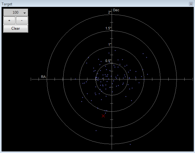
The
target display is another useful way to visualize overall guider
performance. The red 'X' shows the star displacement for the most
recent guide exposure, while the blue dots show the recent history.
You can zoom in or out with the controls at the upper left of the
window, as well as change the number of points shown in the history.
Adaptive Optics (AO) Graph
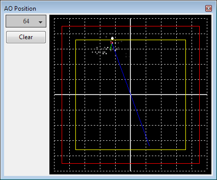
The
AO graph is equivalent to the 'target' display, but shows the history
of corrections relative to the axes of the adaptive optics device.
The red rectangle indicates the outer edges of the AO device,
while the interior yellow rectangle shows the "bump" region. If
the star moves outside the yellow rectangle, PHD2 will send a sequence
of move commands to the mount - the "bump" - to smoothly place the guide star back
near the center position. When this occurs, green and blue lines
will show the incremental bump and the remaining bump respectively.
The white dot on the display shows the current AO position, and
the green circle (red when a bump is in progress) shows the averaged AO position. The button in
the upper left controls how many points will be
plotted in the history.
Dockable/Moveable Graphical Windows
When
the various performance windows are initially displayed, they are
"docked" in the main window. This means they are sized in a
particular way and are aligned with two edges of the window - they are
entirely contained within the bounds of the main PHD2 window.
However, you can move them around and resize them by clicking and
dragging on the title bar of the window you want to examine. This
will often let you get a better view of the details being shown in the
graphs. They can be re-docked by dragging the title bar to the
general region in which you want them docked - bottom, right, etc.
With just a bit of practice, it's easy to place them where they
are most convenient.
There is also a menu item under the 'View" pulldown menu labeled 'Restore
window positions.' Clicking on this menu item will automatically
restore all of the dockable/moveable windows to their default, docked
positions. This can be useful , for example, if you are switching
between screens with different resolutions and one or more of the
dockable windows has been "lost." This function also restores the
main PHD2 window to its default size, with a position near the upper
lefthand corner of the screen.